728x90
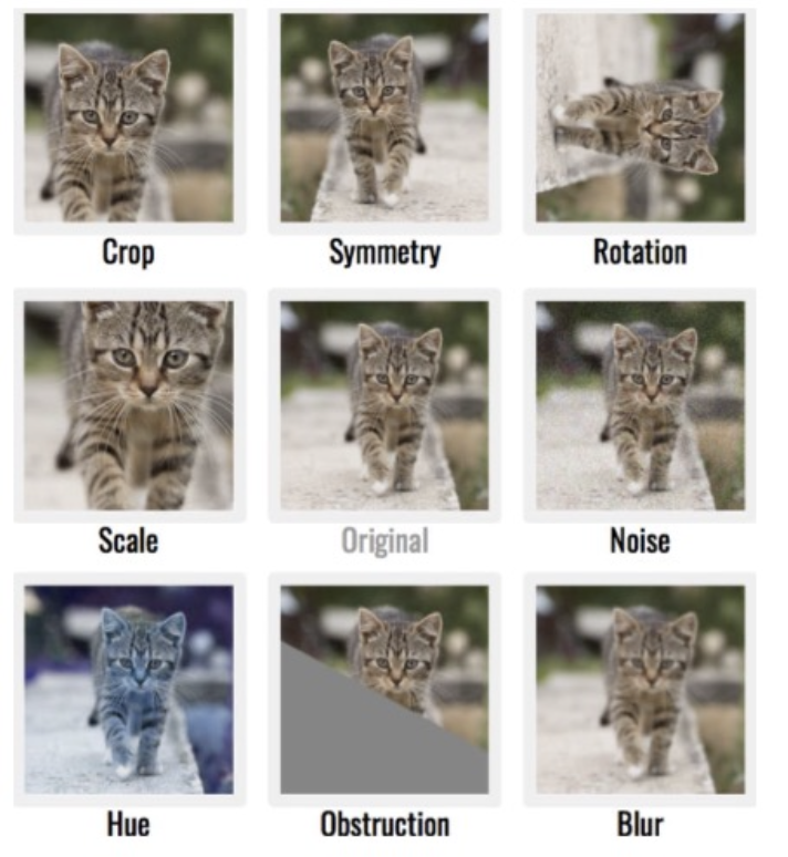
학습데이터를 변형시켜 마치 다른 학습데이터처럼 만들기 : 한장의 사진으로 여러장의 학습데이터를 만들 수 있다.
import cv2
import matplotlib.pyplot as plt
import numpy as np

image = cv2.imread("image02.jpeg")
image = cv2.cvtColor(image, cv2.COLOR_BGR2RGB)
# #### rotation ####
# angle = 30

# h, w = image.shape[:2]
# center = (w//2, h//2)
# M = cv2.getRotationMatrix2D(center, angle, 1.0)
#     # getRotationMatrix2D(중심 좌표, 회전 각도, 크기 변환 비율)

# rotated_img = cv2.warpAffine(image, M, (w, h))
#                 # warpAffine(원본 이미지, 회전 행렬, 이미지 크기)

# plt.imshow(image)
# plt.show()

# plt.imshow(rotated_img)
# plt.show()
# #### rotation ####

#### zoom ####
# h, w = image.shape[:2]

# zoom_scale = 4 # 이미지 확대/축소 배율
# enlarged_img = cv2.resize(image, (w*zoom_scale, h*zoom_scale), interpolation=cv2.INTER_CUBIC)
#             # resize(원본 이미지, (최종 너비, 최종 높이), 이미지 보간 방법 (ex: cv2.INTER_CUBIC))
# center = [enlarged_img.shape[0] // 2, enlarged_img.shape[1] // 2]
# cut_half = 300
# zoomed_img = enlarged_img[center[0]-cut_half:center[0]+cut_half, center[1]-cut_half:center[1]+cut_half]
# plt.imshow(zoomed_img)
# plt.show()
#### zoom ####


#### shift ####

# shift = (0, 50)
# M = np.float32([
#     [1, 0, shift[0]],
#     [0, 1, shift[1]]
# ])
# # 이동 행렬: 좌측 2x2 -> 회전 행렬 (현재 단위행렬), 우측 1열: 이동 행렬 (x 변위, y 변위)

# shifted_img = cv2.warpAffine(image, M, (image.shape[1], image.shape[0]))
# plt.imshow(shifted_img)
# plt.show()
#### shift ####

#### flip ####
# flipped_img_updown = cv2.flip(image, 0) # 상하반전
# flipped_img_leftright = cv2.flip(image, 1) # 좌우반전
# flipped_img_lr_other = cv2.flip(image, -1) # 상하 & 좌우반전

# plt.imshow(image)
# plt.show()
# plt.imshow(flipped_img_updown)
# plt.show()
# plt.imshow(flipped_img_leftright)
# plt.show()
# plt.imshow(flipped_img_lr_other)
# plt.show()
#### flip ####

#### salt-and-pepper noise ####
# noise = np.zeros(image.shape, np.uint8) # uint8 = unsigned int 8-bit (부호 없는 1바이트 정수)
# cv2.randu(noise, 0, 255)
# black = noise < 30 # [True, True, False, False, False, ...] 형태의 Mask 생성
# white = noise > 225
# noise[black] = 0
# noise[white] = 255

# noise_b = noise[:, :, 0] # image.shape (h, w, c) -> h*w*c -> color channel : B, G, R
# noise_g = noise[:, :, 1]
# noise_r = noise[:, :, 2]
# noisy_img = cv2.merge([
#     cv2.add(image[:, :, 0], noise_b),
#     cv2.add(image[:, :, 1], noise_g),
#     cv2.add(image[:, :, 2], noise_r)
# ])

# plt.imshow(image)
# plt.show()
# plt.imshow(noisy_img)
# plt.show()
#### salt-and-pepper noise ####


#### Gaussian Noise ####
# mean = 0
# var = 100
# sigma = var ** 0.5

# gauss = np.random.normal(mean, sigma, image.shape)
# gauss = gauss.astype('uint8')

# noisy_img = cv2.add(image, gauss)

# plt.imshow(noisy_img)
# plt.show()
#### Gaussian Noise ####


#### 색조 변경 ####
# RGB , HSV
# hsv_img = cv2.cvtColor(image, cv2.COLOR_RGB2HSV)
# hue_shift = 30
# hsv_img[:, :, 0] = (hsv_img[:, :, 0] + hue_shift) % 180
# rgb_img = cv2.cvtColor(hsv_img, cv2.COLOR_HSV2RGB)

# plt.imshow(image)
# plt.show()
# plt.imshow(rgb_img)
# plt.show()
#### 색조 변경 ####


#### 색상 변환 ####
# hsv_img = cv2.cvtColor(image, cv2.COLOR_RGB2HSV)

# # hsv[h, w, c]
# hsv_img[:, :, 0] += 50 # Hue -> 50도 증가
# hsv_img[:, :, 1] = np.uint8(hsv_img[:, :, 1] * 0.5)  # 채도
# hsv_img[:, :, 2] = np.uint8(hsv_img[:, :, 2] * 1.5)  # 밝기

# # imshow <- BGR / RGB 로 강제로 디코딩
# rgb_img = cv2.cvtColor(hsv_img, cv2.COLOR_HSV2RGB)
# plt.imshow(rgb_img)
# plt.show()
#### 색상 변환 ####


#### 이미지 크롭 ####
# x, y, w, h = 300, 300, 200, 200  # (100, 100) 좌표에서 (200 * 200) 크기로 자를 것임
# crop_img_wide = image[y-h:y+h, x-w:x+w] # (x, y) 를 중심으로 2w, 2h 크기로 자름
# crop_img_lt = image[y:y+h, x:x+w] # (x, y) 를 기점으로 (w, h) 만큼 오른쪽 아래로 간 크기로 자름

# plt.imshow(image)
# plt.show()
# plt.imshow(crop_img_wide)
# plt.show()
# plt.imshow(crop_img_lt)
# plt.show()
#### 이미지 크롭 ####

#### warpAffine ####
# x_diff = 50
# y_diff = 100
# h, w, c = image.shape
# M = np.float32([
#     [1, 0, x_diff],
#     [0, 1, y_diff]
# ]) # x축으로 50, y 축으로 100 이동하는 병진이동행렬
# shifted_img = cv2.warpAffine(image, M, (w, h))

# M = cv2.getRotationMatrix2D((w // 2, h // 2), 45, 1.0)
# rotated_img = cv2.warpAffine(image, M, (w, h))

# M = cv2.getRotationMatrix2D((w // 2, h // 2), 0, 0.5)
# halfed_img = cv2.warpAffine(image, M, (w, h), flags=cv2.INTER_AREA) # 가장자리를 검은색으로 칠한, 원본 이미지 크기와 같은 축소 이미지
# croped_img = halfed_img[h//2 - h//4 : h//2 + h//4,
#                         w//2 - w//4 : w//2 + w//4] # 가장자리를 잘라낸 이미지

# resized_img = cv2.resize(image, (w//2, h//2), interpolation=cv2.INTER_AREA)
# plt.imshow(image)
# plt.show()
# plt.imshow(shifted_img)
# plt.show()
# plt.imshow(rotated_img)
# plt.show()
# plt.imshow(resized_img)
# plt.show()
# plt.imshow(halfed_img)
# plt.show()
# plt.imshow(croped_img)
# plt.show()
#### warpAffine ####

#### blurring ####
# blur_img = cv2.GaussianBlur(image, (5, 5), 5)

# plt.imshow(blur_img)
# plt.show()
#### blurring ####

#### adaptive threshold ####
# img_gray = cv2.cvtColor(image, cv2.COLOR_RGB2GRAY)

# thresh = cv2.adaptiveThreshold(img_gray, 255, cv2.ADAPTIVE_THRESH_MEAN_C, cv2.THRESH_BINARY, 11, 2)
# # ADAPTIVE_THRESH_MEAN_C: 적응형 임계값 처리, 임계값 기준을 평균치를 사용함
# # 인자 11: 블록 크기, 11x11 블록으로 이미지를 나눈 후 해당 영역
# plt.imshow(img_gray, 'gray')
# plt.show()
# plt.imshow(thresh, 'gray')
# plt.show()
#### adaptive threshold ####


#### 색온도 보정 ####
# org_img = image.copy()
# balance = [0.8, 0.7, 0.8]

# for i, value in enumerate(balance):
#     if value != 1.0:
#         org_img[:, :, i] = cv2.addWeighted(org_img[:,:,i], value, 0, 0, 0)
#                             # addWeighted: src에 대해 value만큼의 가중치로 색온도 조절

# plt.imshow(org_img)
# plt.show()
#### 색온도 보정 ####


#### 모션 블러 ####
# kernal_size = 15
# kernal_direction = np.zeros((kernal_size, kernal_size))
# kernal_direction[int((kernal_size)//2), :] = np.ones(kernal_size)
# kernal_direction /= kernal_size # 커널의 합이 1이 되도록
# kernal_matrix = cv2.getRotationMatrix2D((kernal_size/2, kernal_size/2), 45, 1)
# kernal = np.hstack((kernal_matrix[:, :2], [[0], [0]]))
#         # kernal_matrix[:, :2] <- 회전 행렬에서 병진이동 벡터를 제외하고 회전 행렬 값만 가져옴
#         # [[0],[0]] <- 병진이동 벡터 (이동 X)
# kernal = cv2.warpAffine(kernal_direction, kernal, (kernal_size, kernal_size))

# motion_blur_img = cv2.filter2D(image, -1, kernal)
# plt.imshow(motion_blur_img)
# plt.show()
#### 모션 블러 ####


#### 난수 노이즈 ####
# gray_img = cv2.imread('image02.jpeg', cv2.IMREAD_GRAYSCALE)
# h, w = gray_img.shape

# mean = 0
# var = 100
# sigma = var ** 0.5

# gaussian = np.random.normal(mean, sigma, (h, w))
# noisy_image = gray_img + gaussian.astype(np.uint8)
# # uint8 -> 0 ~ 255
# cv2.imshow("", noisy_image)
# cv2.waitKey()
#### 난수 노이즈 ####

#### 채도 조정 ####
# img = cv2.imread('image02.jpeg')
# org_img = img.copy()

# img_hsv = cv2.cvtColor(img, cv2.COLOR_BGR2HSV)
# saturation_factor = 1.5
# img_hsv[:, :, 1] = img_hsv[:, :, 1] * saturation_factor

# saturated_img = cv2.cvtColor(img_hsv, cv2.COLOR_HSV2BGR)

# cv2.imshow("", org_img)
# cv2.waitKey()
# cv2.imshow("", saturated_img)
# cv2.waitKey()
#### 채도 조정 ####


#### 밝기 조정 ####
# img = cv2.imread('image02.jpeg')
# org_img = img.copy()

# bright_diff = 50
# img_brighten = cv2.convertScaleAbs(img, alpha=1, beta=bright_diff)

# cv2.imshow("org", org_img)
# cv2.imshow("brighten", img_brighten)
# cv2.waitKey()
#### 밝기 조정 ####

#### 노이즈 제거 ####
# img_filtered = cv2.medianBlur(image, 5)
# plt.imshow(image)
# plt.show()
# plt.imshow(img_filtered)
# plt.show()
#### 노이즈 제거 ####

#### 히스토그램 균일화 ####
# img_gray = cv2.imread("image02.jpeg", cv2.IMREAD_GRAYSCALE)
# img_equalized = cv2.equalizeHist(img_gray)

# cv2.imshow("org", img_gray)
# cv2.imshow("hist_equal", img_equalized)
# cv2.waitKey()
#### 히스토그램 균일화 ####
728x90
'AI > [Preprocessing]' 카테고리의 다른 글
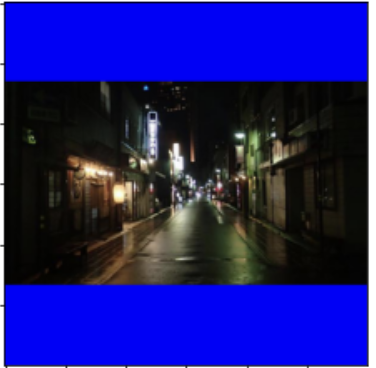
| [전처리] 이미지 비율에 맞게 정사각형 만들기 (0) | 2023.06.15 |
|---|---|
| [전처리] 가져온 사진 정보 받기 (feat, xml) (1) | 2023.06.15 |
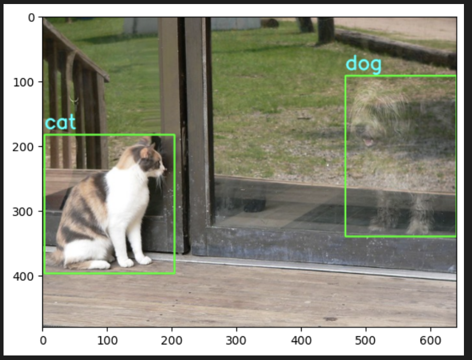
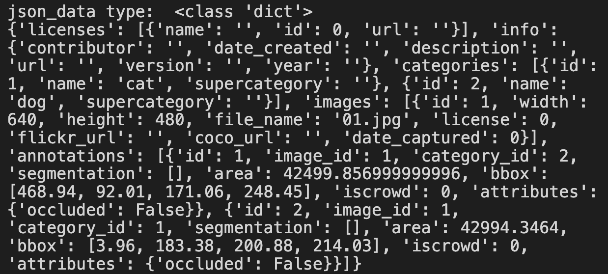
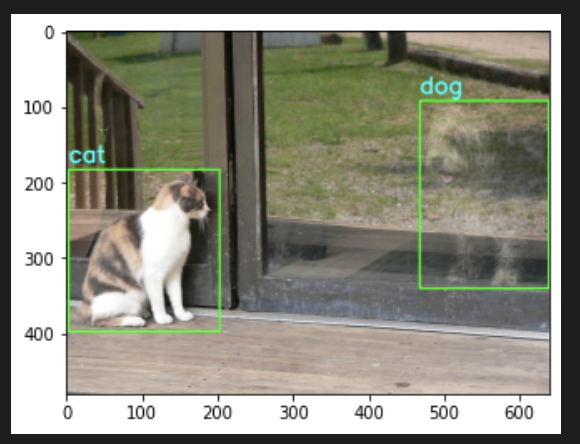
| [전처리] 가져온 사진 정보 받기 (feat, json) (0) | 2023.06.14 |
| [전처리] 폴더에 있는 사진 가져오기 (0) | 2023.06.14 |
| [전처리] 범주형 데이터 전처리 (0) | 2023.06.06 |